
Data Analysis
9 min
How to Recover When Your CSV Upload Fails
A practical CSV upload recovery workflow for file size, encoding, delimiters, headers, malformed rows, validation, and safe re-upload.
Read More


It can be challenging to identify significant patterns in data rows and columns. You are not alone if you have devoted hours to creating charts, manually adding numbers, or applying conditional formatting in Excel. What's the good news? This laborious process can be completed in a matter of seconds with quick analysis tool excel.
With the help of quick analysis tool excel, you can view, format, and compute data in real time. With a single click or keyboard shortcut, you can quickly add conditional formatting, create charts, add totals, create tables, and add sparklines. You don't even have to write a formula or navigate through several ribbon menus.
Since its addition to Excel in 2013, the quick analysis tool in excel has fundamentally altered how users engage with their data. Searching through menus and dialog boxes is no longer necessary. Numerous real-time analysis options are immediately available for you to view and utilize. Whether you're a student reviewing research data, a sales manager monitoring team performance, or a business analyst creating monthly reports, this tool can save meaningful time on the routine parts of data analysis — the formatting, charting, and quick summaries that would otherwise eat half your afternoon.
Everything you need to know about the quick analysis tool will be covered in this comprehensive guide. We will discuss: The Quick Analysis tool's definition and operation; thorough instructions for utilizing and accessing each feature; sophisticated methods for utilizing multiple analysis features simultaneously; real-world examples and use cases from various industries; and when to use AI-powered tools like Anomaly AI versus Excel's built-in tools for larger datasets.
After completing this lesson, you will be able to transform unstructured data into actionable knowledge in a matter of minutes rather than hours. First, let's examine the other features of Excel's Quick Analysis tool.
Microsoft Excel's Quick Analysis tool provides instant access to data analysis options. Unlike other Excel features that require navigating through numerous menus and ribbons, quick analysis tool in excel makes it simple to see everything you need in one location.
The tool is made up of five primary functions:
Formatting: Conditional formatting rules like data bars, color scales, and icon sets to identify patterns and outliers.
Charts: Create scatter plots, pie charts, line graphs, and column charts with a single click.
Totals: Add up, calculate averages, count, determine percentages, and maintain running totals without formulas.
Tables: Convert data ranges into structured Excel tables with filtering and sorting tools.
Sparklines: Create in-cell charts that provide a succinct overview of trends for dashboards and reports.
First, select your data range (at least two cells). Include column headers for best results. There are three ways to access quick analysis tool in excel:
Method 1: Quick Analysis Button - After selecting data, click the lightning bolt icon that appears at the bottom-right corner of your selection.
Method 2: Keyboard Shortcut - Press Ctrl + Q (Windows) or Control + Q (Mac) after selecting your data.
Method 3: Right-Click Menu - Right-click on your selected data and choose Quick Analysis from the context menu.
Now that you understand how to use the quick analysis tool, it's time to discover why it's so helpful. The tool has five distinct tabs, each of which focuses on a distinct kind of data analysis. This section will cover every feature in great detail, including how it functions, when to use it, and how it can transform your raw data into information that is useful.
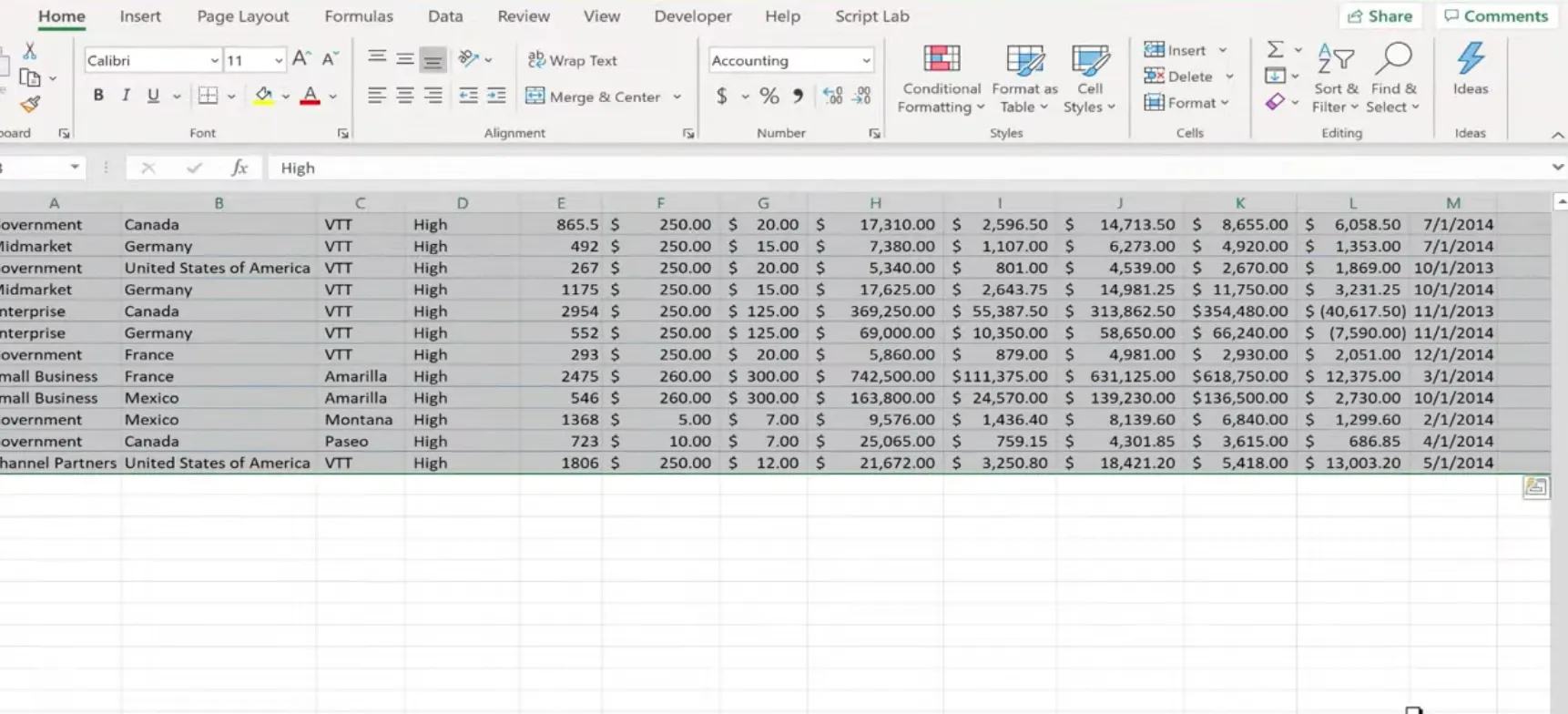
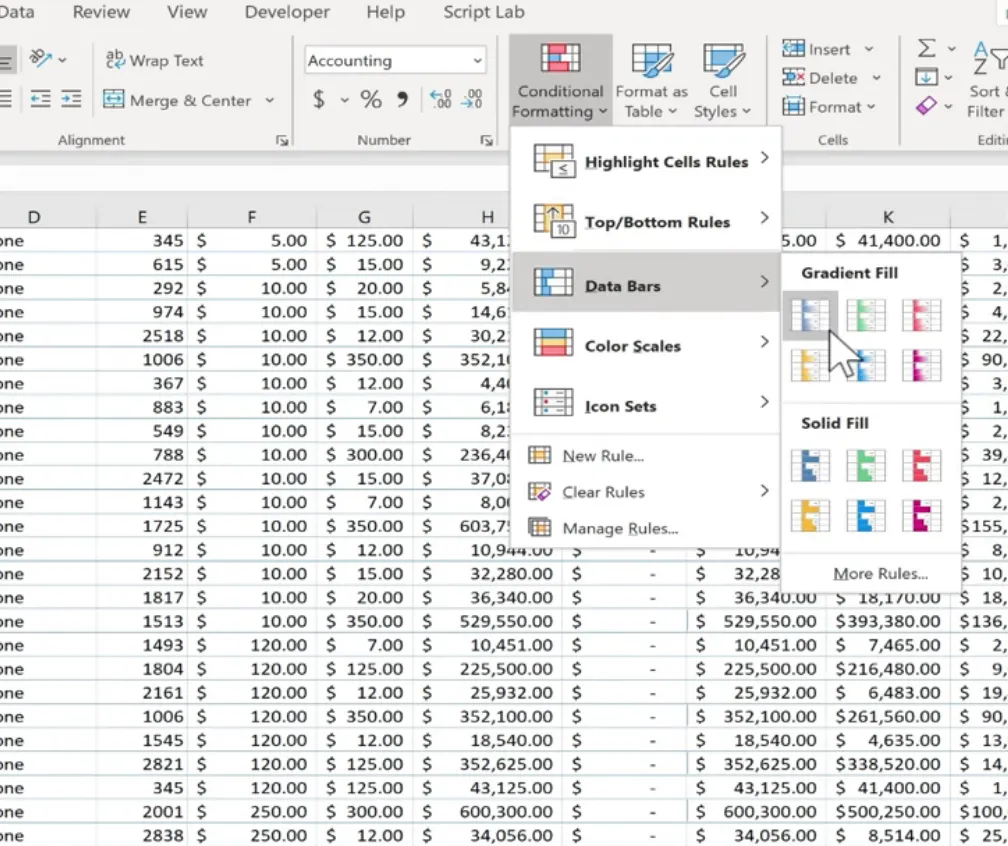
The Formatting tab applies conditional formatting to visually analyze data with a single click:
Data Bars: Horizontal bars appear within cells, with length proportional to cell values. Perfect for comparing sales figures, budget distribution, or performance metrics at a glance.
Color Scales: Gradient colors across your data range create heat map effects. Ideal for financial dashboards, quality control data, and survey results.
Icon Sets: Small symbols (arrows, flags, circles) display status while keeping numbers visible. Great for KPIs, project status dashboards, and inventory control.
Greater Than and Top 10%: Automatically highlights outliers and top performers—excellent for identifying peak performance and highest values.
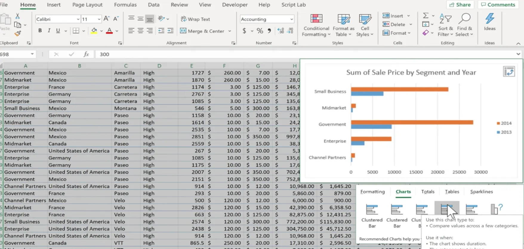
The Charts tab automatically recommends the most appropriate visualizations based on your data structure:
Clustered Column Charts: Compare values between groups. Perfect for showing monthly sales by product line or performance across categories.
Stacked Column Charts: Display both individual values and totals. Ideal for budget breakdowns and market share composition.
Line Charts: Show trends over time like stock prices, website traffic, or seasonal patterns.
Pie Charts: Illustrate proportional relationships. Best used with 5 or fewer categories for demographic or budget views.
Scatter Plots: Examine relationships between two variables like advertising spend vs. sales or correlations in experimental data.
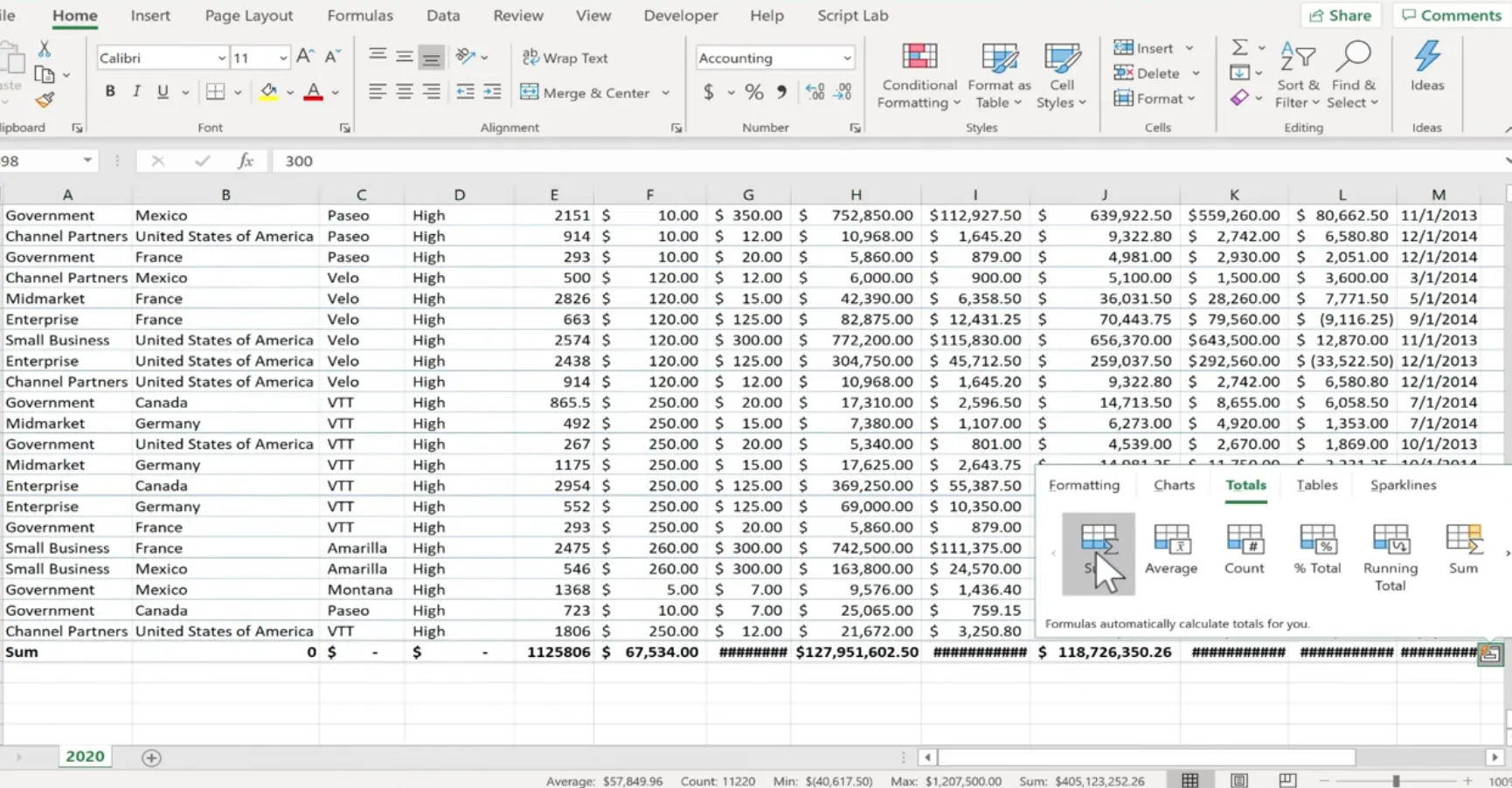
Get instant calculations without writing formulas. Excel inserts real formulas that update automatically:
Sum: Automatically adds totals for columns and rows. Essential for revenue, expenses, and financial calculations.
Average: Calculates averages for test results, performance indicators, and measurements (ignores text and empty cells).
Count: Counts numbers, text entries, or non-empty cells for tracking participation rates and inventory.
% Total: Converts values into percentages of the grand total for analyzing territory performance and channel contributions.
Running Total: Creates cumulative sums for tracking cash flow and progress toward goals.
Convert data ranges into structured Excel tables with one click. Tables provide:
• Automatic alternating row colors for easier reading
• Filter buttons in headers for instant sorting and filtering
• Structured references using column names (=SUM(Sales[Amount]) instead of =SUM(B2:B100))
• Auto-formatting for new rows with formulas that expand automatically
• Built-in aggregate functions (sum, average, count, max, min) via total rows
Sparklines are tiny in-cell charts that display trends without taking up worksheet space. Perfect for compact dashboards:
Line Sparklines: Mini line charts showing changes over time—ideal for stock performance, seasonal patterns, and growth trends.
Column Sparklines: Tiny column charts displaying individual data points. Great for weekly production or monthly sales tracking.
Win/Loss Sparklines: Show binary outcomes with bars above/below baseline. Perfect for tracking performance above or below targets.
Let's walk through a practical example using monthly sales data by region to demonstrate how quick analysis tool in excel transforms raw data into insights.
Ensure your data is organized in a clear table format with headers in the first row and consistent data types in each column. Remove any empty rows or columns within your data range.
Click on the first cell of your data (including headers) and drag to the last cell, or click the first cell and press Ctrl+Shift+End to select to the end of your data.
Click the Quick Analysis icon that appears at the bottom-right corner of your selection, or press Ctrl+Q.
Click the Formatting tab and hover over Data Bars to preview how bars will appear in your cells. Click to apply, and Excel adds visual bars that make it easy to compare values at a glance.
Click the Charts tab and hover over different chart types. Select Clustered Column to create a chart comparing sales across regions and months. The chart appears instantly and updates automatically if you change your data.
Click the Totals tab and select Sum to add row and column totals. Hover your cursor over 'Sum' in the column options to view the total sales by region. Excel creates a new row beneath your data with SUM formulas that determine the total for each region for the quarter when you click 'Apply.' These formulas will automatically update if you make any changes to the monthly values.
The total sales for each month across all regions can then be viewed by moving your mouse over 'Sum' in the row options. Excel will add a column displaying the monthly totals if you click 'Apply.' Now, you can see which region had the largest influence on quarterly performance and which month generated the highest total revenue.
Excel's quick analysis tool enters actual formulas rather than fixed values, as demonstrated by the Totals feature. Click on any cell in the total to see how Excel calculated that amount. This openness helps you learn Excel formulas while still being able to insert them quickly.
With the quick analysis tool, you can now finish your sales analysis in less than two minutes. It provides you with calculated totals, visual charts, and formatted data.
Before you can use Excel's analysis tools, you must first complete the manual cleaning requirements. Excel's quick analysis tool assumes that your data is already clean and in the correct format. It is rare for real-world data to arrive in perfect condition. Duplicates, inconsistent dates, missing values, text mingled with numbers, and numerous other problems will be present. Cleaning up large datasets by hand using Excel formulas and filtering can take hours or even days.
The majority of the laborious analysis still needs to be done by you because of the limited AI-powered insights. Excel's quick analysis tool can assist you in formatting and charting your data according to basic guidelines for data setup, but it isn't very knowledgeable about the meaning of your data.
There is no automated anomaly detection, so you have to manually examine the data or create complex formulas to identify outliers. You can determine statistical thresholds, manually create conditional formatting rules, or simply ignore the issues.
Workflow is slowed down by static analysis vs. dynamic dashboards. Charts created and formatted with Excel's analytics tools are static outputs. If you alter the data that your analysis is based on, you will need to either manually refresh it or redo it. There isn't a dashboard that continuously monitors your data, notifies you of changes, or allows stakeholders to view various perspectives in real time.
Step 1: Upload Your Data - Anomaly AI accepts Excel files (.xlsx, .xls), CSV files, and direct connections to cloud databases like BigQuery, MySQL, and Snowflake. The platform handles millions of rows that would overwhelm Excel, with automatic file validation and data type detection.
Step 2: Automated Data Cleaning - AI-powered tools handle duplicate removal, text and date normalization, and outlier detection. The platform distinguishes between data errors and legitimate extreme values, flagging anomalies like unusual sales patterns or unexplained expense increases for your review.
Step 3: Intelligent Data Transformation - The analytics engine automatically discovers patterns and relationships in your data, calculates relevant KPIs (growth rates, moving averages, efficiency ratios), and provides statistical summaries including distributions and quality scores—all without requiring formulas or coding.
Step 4: Interactive Dashboard Creation - Auto-generated dashboards feature appropriate visualizations based on your data type, drill-down analytics for detailed exploration, real-time filtering, and responsive design. Share dashboards with stakeholders or export to Excel, PowerPoint, or PDF formats.
Quick analysis tool in excel transforms the way you handle data. With the help of this robust feature, you can quickly perform calculations, create engaging graphs, and format documents professionally without having to be an Excel guru. Excel's quick analysis tool greatly expedites your work, whether you're creating dashboards, financial reports, or examining sales trends.
However, you might want to upgrade to AI-powered platforms like Anomaly AI if your datasets grow or your analysis requirements become more complex. These tools perform the laborious analysis tasks that Excel's built-in features cannot, such as automated cleaning, pattern recognition, and interactive dashboards.
Experience AI-driven data analysis with your own spreadsheets and datasets. Generate insights and dashboards in minutes with our AI data analyst.
Founder, Anomaly AI (ex-CTO & Head of Engineering)
Abhinav Pandey is the founder of Anomaly AI, an AI data analysis platform built for large, messy datasets. Before Anomaly, he led engineering teams as CTO and Head of Engineering.
Continue exploring AI data analysis with these related insights and guides.
A practical CSV upload recovery workflow for file size, encoding, delimiters, headers, malformed rows, validation, and safe re-upload.

A precise guide to the five advanced Excel workflows where Anomaly AI is faster than pivot tables, and where Excel still wins.

A workbook-safety workflow for analyzing .xls and .xlsx files with AI: sheets, headers, formulas, hidden data, sensitive fields, and reviewable outputs.